GisSOM for Clustering Multivariate Data ‒ GisSOM
This is the last blog of the three-part series aiming at introducing GisSOM, a self-organizing maps (SOM) software especially designed to handle spatially referenced data. If you are not acquainted with the subject, it would be useful to read the two previous parts of the blog series first. Two SOM-related terms used later are important to remember: Best-matching unit (BMU) is the node on SOM grid where a particular data point is assigned to and codebook vector is a SOM node vector. The codebook vector elements correspond to the variables in the input data.
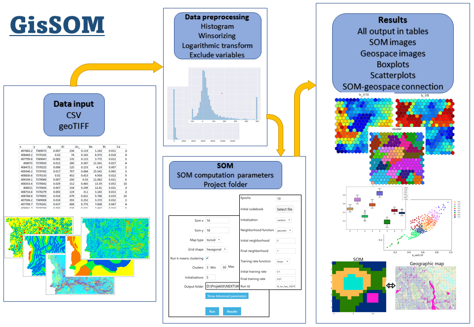
GisSOM (Figure 1) was developed in the New Exploration Technologies (NEXT) project (ended in September, 2021) which aimed at developing new geological models, sensitive exploration technologies and data analysis methods for mineral exploration. The role of GisSOM in this context is in preprocessing and exploring the multivariate datasets that are generated from geoscientific measurements and observations. The core of GisSOM is the computation of self-organizing maps, which is accompanied by k-means clustering and many auxiliary functions for preprocessing input data and visualizing the SOM and k-means clustering results. GisSOM has a user interface that provides an easy access to all its functionalities. What probably interests you the most are the results you get from GisSOM. These will be presented shortly, right after a brief description of preparing the input data and starting the SOM computation.
Data Input and Preprocessing with GisSOM
GisSOM accepts data as text files with comma separated values (CSV) and as georeferenced TIF files. TIF files are often used when working with spatial gridded data (rasters, maps), while the CSV format can accommodate any kind of dataset; spatial or non-spatial, gridded or not gridded. CSV format can also include labelled data. For instance, if you wish to classify a satellite image to regions representing “cloud”, “field”, “forest”, “water”, you can provide this information for the pixels with known class.
The input dataset is probably already preprocessed in many ways, but in GisSOM, there are also functions that are often needed to ensure successful SOM processing: logarithmic transform and winsorizing. These functions are applied for peaked distributions to emphasize differences near the median and to squeeze the long tails. GisSOM shows the histogram of each variable to facilitate making the choice of the transformation function.
SOM Computation
Once you have generated the dataset for SOM analysis, you need to define the parameters for SOM computation. The parameters are separated in two sections: basic and advanced. For basic parameters, you rarely can accept the default values. SOM result is especially sensitive to the size and shape of SOM, the choice of which depends strongly on the number of variables and data points as well as on the distributions of the variables. The best practice to find a suitable set of parameters is trial, trial and trial.
Presentation of the Results
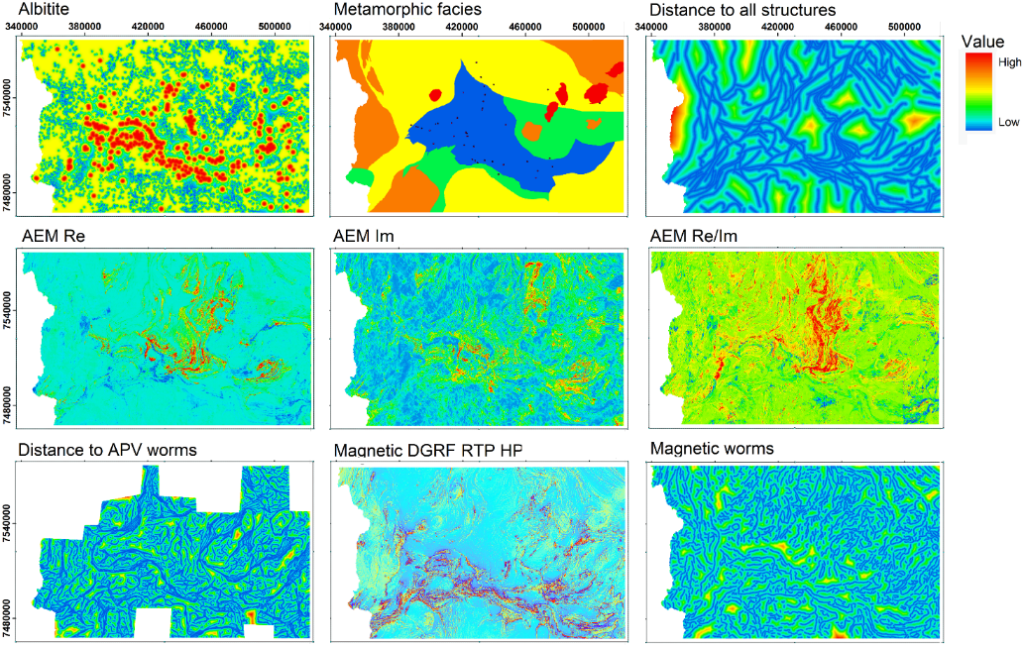
Since the variety of ways of presenting the SOM result is the strength of GisSOM, example results will be presented highlighting some patterns and relations revealed by the results. The input dataset (Figure 2) was generated for prospectivity modelling of orogenic gold deposits in the Central Lapland Greenstone Belt (Torppa et al., 2019). Explaining all the nine variables in the dataset is not relevant, but let’s briefly describe the three that are used in the following example result images. The Albitite map represents a quantity weighted by distance to albitite occurrences and non-occurrences, Metamorphic facies map represents the metamorphic grade and AEM Re is the in-phase component of the electromagnetic response. The data also includes known orogenic gold occurrences in form of labelled data points that are used in this demonstration to label the clusters obtained from SOM and k-means. Labelled data points are shown in (Figure 2) on the map of metamorphic facies.
In GisSOM, the results are shown as figures and plots divided onto six tabs. Four tabs present the results as static figures on SOM grid and in geographic frame, and as boxplots and scatterplots. One tab is for performing k-means clustering for the SOM result and one tab for investigating the relation of the SOM grid to the geographic frame. In addition, all the information needed to generate the visualizations are provided as text files for further use in other applications.
Results on SOM Grid
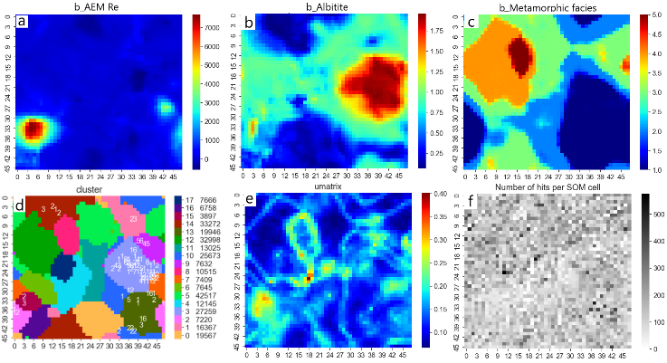
On SOM grid (Figure 3), GisSOM shows the k-means clusters, distribution of each variable separately, U-matrix and the number of data points assigned to each SOM node (hits). Three variables are shown as examples (Figure 3a-c). For instance, when compared to the k-means cluster map with labelled data points marked (Figure 3d), it is obvious that high albitite value together with low metamorphic facies value is favorable for the occurrence of gold. The U-matrix (Figure 3e) shows the spatial gradient on SOM grid, providing information on the clarity of boundaries between different populations (clusters) in the data. These boundaries are revealed only if there are enough nodes in the SOM grid. Many of the clusters in our example have clear boundaries but, for instance, the cluster representing large AEM Re values is not very well constrained based on the strong variation in the U-matrix.
Results in Geographic Frame
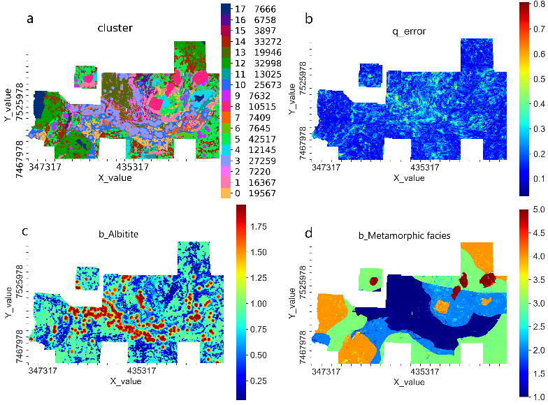
If the input data is spatially referenced, GisSOM shows in geographic frame (Figure 4) the k-means clusters, quantization error and the BMU value for each input variable. High quantization error (Figure 4b) for a data point suggests that there are one or more variables that have anomalous values not retained on SOM. Such data points may be scientifically interesting if the anomaly is not caused by erroneous data. The areas of high quantization error also show a big difference between the original data and the corresponding BMU values for the anomalous variables.
Boxplots and Scatterplots
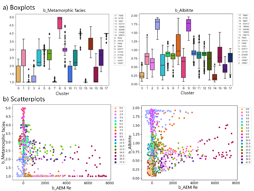
The distribution of each variable on SOM is presented cluster-wise as boxplots. This is one way to investigate quickly how well k-means clustering has performed: clustering has been successful if there are clear differences between the distributions of different clusters. In the example boxplots for albitite and metamorphic facies the difference is obvious (Figure 5a).
The idea of the scatterplots is to show if different clusters show different relations between pairs of variables. The points in the plot are colored based on the cluster that they belong to. As an example, we show scatterplots for albitite and metamorphic grade vs AEM Re (Figure 5b). It is clear, for instance, that high AEM Re and albitite map values occur only in a few clusters, and that there are no high AEM Re values for locations with high metamorphic grade.
K-means Clustering Tab
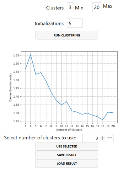
The default clustering result chosen by GisSOM may not be the best clustering scheme for your data. In the k-means clustering tab (Figure 6), you can run the clustering for a selected range of clusters, inspect the Davies-Bouldin indices for each number of clusters, and select for output the number of clusters that best serves your purposes.
SOM vs Geographic Frame
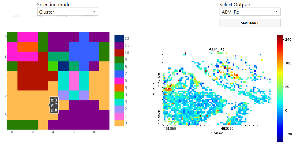
If input data is spatially referenced, the relation between SOM and geographic frame can be interactively investigated (Figure 7). By choosing a cluster or SOM node on the SOM grid (left), the corresponding data points are highlighted in the geographic frame (right). This helps to understand how the original data points are distributed on SOM grid and in the k-means clusters. The background map on the right side can represent either the k-means clusters or any of the input variables.
Could you become a GisSOM user?
Majority of the work in GisSOM development has been done, in addition to the author, by Sakari Hautala with contribution also from Bijal Chudasama and Jaakko Madetoja at the Geological Survey of Finland (GTK). With excellent teamwork, this software tool has become something useful for both scientific research and for generating data products by data producing companies. What is needed now, is feedback from the user community to be able to make the software applicable to a wider range of different use cases. With the information provided in this three-part blog series GisSOM for Clustering Multivariate Data, you can judge whether SOM would be a suitable method to analyze your data, and whether GisSOM is worth giving a try.
Previous blog posts in this three part series are: GisSOM for Clustering Multivariate Data ‒ Multivariate Clustering and a Glance to Self-organizing Maps and GisSOM for Clustering Multivariate Data ‒ Self-organizing Maps. The topics covered in the series, along with an introduction to using SOM for prospectivity modelling of orogenic gold deposits (Chudasama et al., 2021), are addressed in Torppa et al. (2021).
GisSOM installation package, user manual and technical specification document can be found in GitHub.
The research related to this blog series has received funding from the European Union’s Horizon 2020 research and innovation programme under Grant Agreement No. 776804 – H2020-SC5-2017 NEXT – New Exploration Technologies.
Text:
Johanna Torppa, Senior Specialist, Information Solutions, Geological Survey of Finland, johanna.torppa@gtk.fi
References:
Chudasama B., Torppa J., Nykänen V. and Kinnunen J., 2021. Target-scale prospectivity modeling for gold mineralization within the Rajapalot Au-Co project area in northern Fennoscandian Shield, Finland. Part 2: Application of self-organizing maps and artificial neural networks for exploration targeting, Ore Geology Reviews (submitted).
Torppa J., Nykänen V. and Molnár F., 2019. Unsupervised clustering and empirical fuzzy memberships for mineral prospectivity modelling, Ore Geology Reviews 107, pp 58-71.
Torppa J., Chudasama B., Hautala S. and Kim YongHwi, 2021. GisSOM for clustering multivariate data, Geological Survey of Finland, Open File Research Report, 52.